Solving mazes with PDEs instead of AI
FeenoX Tutorial #2
Table of contents
1 Foreword
Welcome the the Second Feenox tutorial, very much inspired on Donald Knuth’s Selected Papers on Fun and Games. And a little bit on Homer Simpson.

Say you want to solve a maze drawn in a restaurant’s placemat: one where both the start and end points are known beforehand as shown in fig. 1. Nowadays the first instinctive reaction would be to fire some fancy AI or ML algorithm. But we are actual engineers and we do value nice maths hacks, don’t we? In order to avoid falling into the alligator’s mouth, we can exploit the ellipticity of the Laplacian operator to solve any maze—even hand-drawn ones. Just FeenoX and a bunch of standard open source tools to convert a bitmapped picture of the maze into an unstructured mesh.
A couple of LinkedIn posts to see some comments and discussions:
- https://www.linkedin.com/feed/update/urn:li:activity:6831291311832760320/
- https://www.linkedin.com/feed/update/urn:li:activity:6973982270852325376/
Other people’s maze-related posts:
- https://www.linkedin.com/feed/update/urn:li:activity:7117082910381232128/
- https://www.linkedin.com/feed/update/urn:li:activity:6972370982489509888/
- https://www.linkedin.com/feed/update/urn:li:activity:6972949021711630336/
- https://www.linkedin.com/feed/update/urn:li:activity:6973522069703516160/
- https://www.linkedin.com/feed/update/urn:li:activity:6973921855275458560/
- https://www.linkedin.com/feed/update/urn:li:activity:6974663157952745472/
- https://www.linkedin.com/feed/update/urn:li:activity:6974979951049519104/
- https://www.linkedin.com/feed/update/urn:li:activity:6982049404568449024/
1.1 Executive summary
We will…
Create and download a random maze online.
Create a FEM mesh for the aisle of the maze (the walls will be the boundary of the domain) using Gmsh.
Solve \nabla^2 \phi(x,y) = 0 subject to the following boundary conditions:
\begin{cases} \phi(x,y) = 1 & \text{at the inlet} \\ \phi(x,y) = 0 & \text{at the outlet} \\ \frac{\partial \phi}{\partial n} = 0 & \text{everywhere else} \\ \end{cases}
PROBLEM laplace 2D
READ_MESH maze.msh

BC start  phi=0
BC end    phi=1

SOLVE_PROBLEM
Show the solution of the maze given by \nabla \phi, properly scaled, in Gmsh:
# write the norm of gradient as a scalar field
# and the gradient as a 2d vector into a .msh file
 WRITE_MESH maze-solved.msh \
     sqrt(dphidx(x,y)^2+dphidy(x,y)^2) \
     VECTOR dphidx dphidy 0
As a bonus, we will also solve a transient case to see how Laplace “tries” all the paths and only keeps the ones that do not find any dead end.
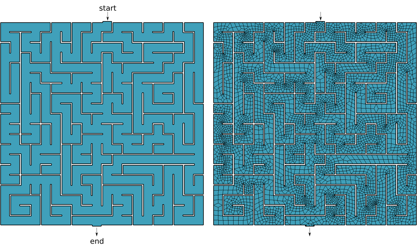
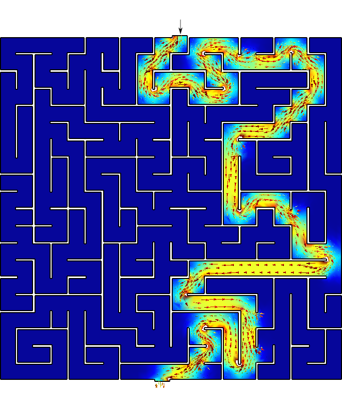
Figure 2: Bitmapped, meshed and solved mazes.. a — Bitmapped maze from https://www.mazegenerator.net (left) and 2D mesh (right), b — Solution to found by FeenoX (and drawn by Gmsh)
2 Creating the mesh
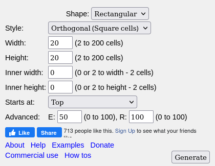
Choose shape, style, width, height, etc. and create a maze
Download it in PNG (fig. 2 (a))
Perform some manipulations and conversions. We are going to need a bunch of free an open source tools:
sudo apt-get install imagemagick potrace inkscape pstoedit make g++Invert the PNG and convert it to PNM with
convertso the aisles are black and the walls are white:convert maze.png -negate maze_negated.pnm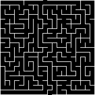
Vectorize the negated bitmap into an SVG with
potrace:potrace maze_negated.pnm --alphamax 0 --opttolerance 0 -b svg -o maze.svg
Convert the SVG to EPS with
inskcapeinkscape maze.svg --export-eps=maze.epsConvert the EPS to DXF with
pstoeditpstoedit -dt -f 'dxf:-polyaslines -mm' maze.eps > maze.dxfConvert the DXF to a Gmsh’s
.geowithdxf2geo(a C++ tool that comes with Gmsh)make dxf2geo ./dxf2geo maze.dxf 0.1
The tutorial directory contains a convenience script to perform all these steps in a single call. Just name your PNG
maze.pngand run./png2geo.sh.The last file
maze.geocontains only lines with the walls of the maze. We need to tell FeenoX where the maze starts and where it ends. Open it with Gmsh:gmsh maze.geo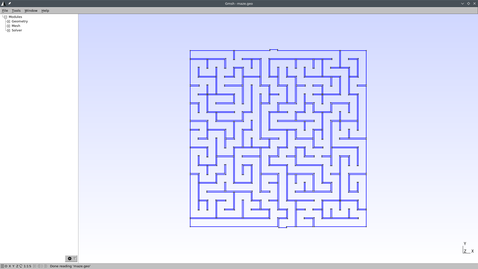
We have to
Add a surface for the aisles of the maze (i.e. the 2D domain where we will apply the Laplace operator):
In the left-pane tree, go to Geometry \rightarrow Elementary entities \rightarrow Add \rightarrow Plane Surface.
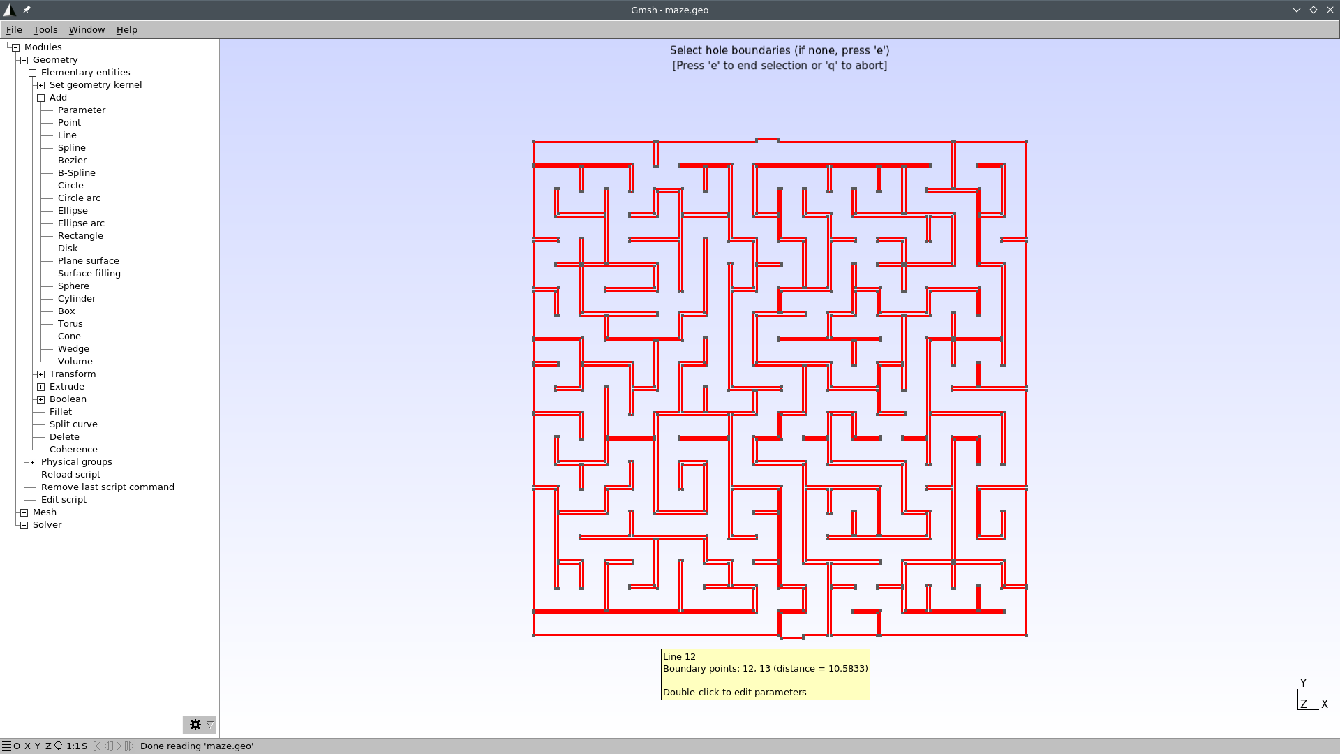
When prompted to “select surface boundary” click on any of the blue edges. They all should turn to red:
Press
eto end selection andqto exit the selection mode.Press
2to make a preliminary 2D mesh to see if it worked: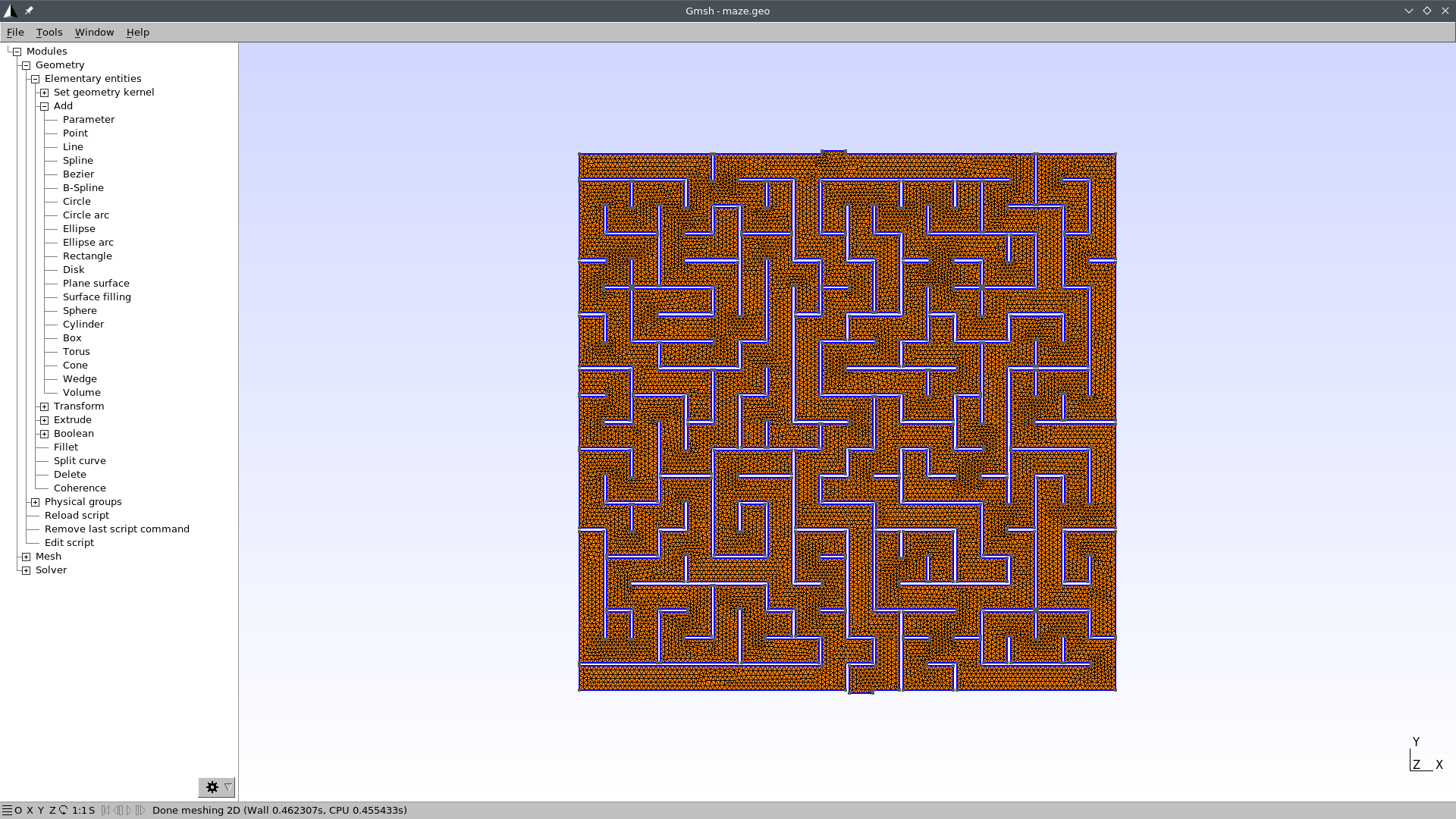
Go to Geometry \rightarrow Physical groups \rightarrow Add \rightarrow Surface.
When prompted to “select surfaces” click on any point of the maze. The mesh should turn red:
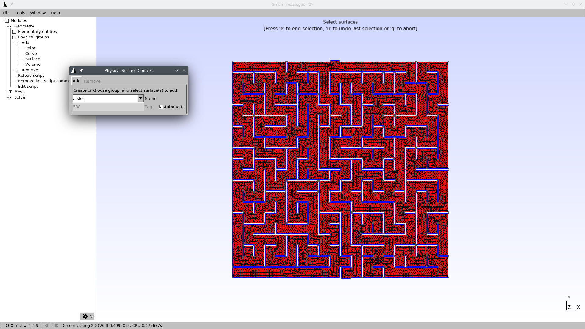
Write “aisles” as the group’s name.
Press
eto end the selection. You might need to click somewhere in the Gmsh window so as to get the focus out of the name text field.Press
qto exit the selection mode.Press
0to reload themaze.geofile and remove the temporary mesh.
Set physical curves for “start” and “end” (i.e. the 1D edges that will hold the Dirichlet boundary conditions)
In the left-pane tree, go to Geometry \rightarrow Physical groups \rightarrow Add \rightarrow Curve.
When prompted to “select curves” click on the edge (or edges) that define the inlet.
Write “start” as the group’s name.
Press
eto end the selection. You might need to click somewhere in the Gmsh window so as to get the focus out of the name text field.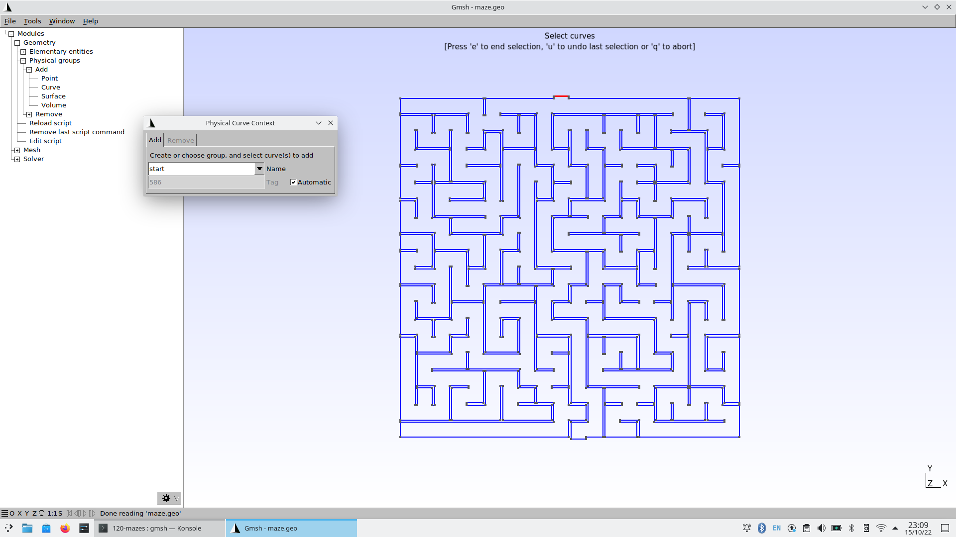
Do the same thing for the outlet, and name it “end.” Alternatively, find out the edge id of the outlet by zooming in a little bit into the outlet and then going to Tools \rightarrow Options \rightarrow Geometry \rightarrow Curve Labels:
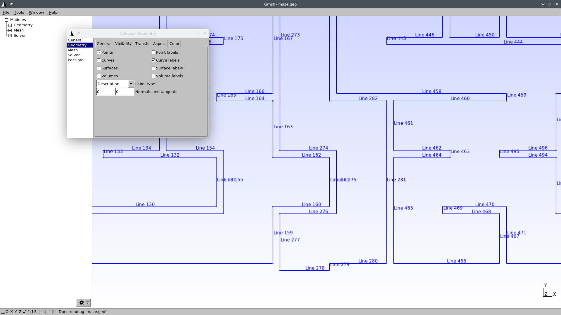
In this case, the curve id is 278. So we can edit the file
maze.geoand add this line at the very end:Physical Curve("end") = {278};Now our
maze.geocontains a proper definition of the domain where we will solve \nabla^2 \phi = 0.
Create the actual mesh
maze.mshout ofmaze.geogmsh -2 maze.geo
3 Solving the steady-state Laplace equation
We have to solve \nabla^2 \phi = 0 with the following boundary conditions
\begin{cases} \phi=0 & \text{at “start”} \\ \phi=1 & \text{at “end”} \\ \nabla \phi \cdot \hat{\mathbf{n}} = 0 & \text{everywhere else} \\ \end{cases}
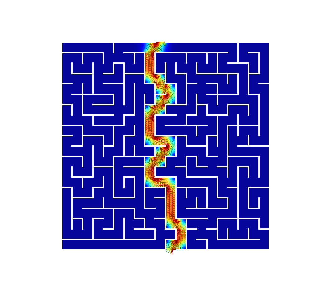
The solution to the maze is given by the gradient of the solution \nabla \phi.
This translates into FeenoX to the following input file:
PROBLEM laplace 2D  # pretty self-descriptive, isn't it?
READ_MESH maze.msh

# boundary conditions (default is homogeneous Neumann)
BC start  phi=0
BC end    phi=1

SOLVE_PROBLEM

# write the norm of gradient as a scalar field
# and the gradient as a 2d vector into a .msh file
WRITE_MESH maze-solved.msh \
    sqrt(dphidx(x,y)^2+dphidy(x,y)^2) \
    VECTOR dphidx dphidy 0
Let us break the WRITE_MESH
instruction up. The resulting mesh name is maze-solved.msh.
It cannot be the same maze.msh we used as the input
mesh.
Those aisles that go into dead ends are expected to have a very small
gradient, while the aisles that lead to the exit are expected to have a
large gradient. The solution \phi(x,y)
is mapped into a function phi(x,y). Its gradient
\nabla \phi =
\begin{bmatrix}
\frac{\partial \phi}{\partial x} \\
\frac{\partial \phi}{\partial y}
\end{bmatrix}
is mapped into two scalar functions, dphidx(x,y)
and dphidy(x,y). So we write a scalar field with the
magnitude of the gradient \nabla \phi
as sqrt(dphidx(x,y)^2+dphidy(x,y)^2)(remember that
everything is an expression, including the fields written in the
post-processing files). We also write the gradient itself as a vector so
we can follow the arrows from the start down to the end.
$ feenox maze.fee
$
That’s it. Remember the Unix rule of silence.
4 Results
Open maze-solved.msh with Gmsh:
gmsh maze-solved.mshYou should see something like this:
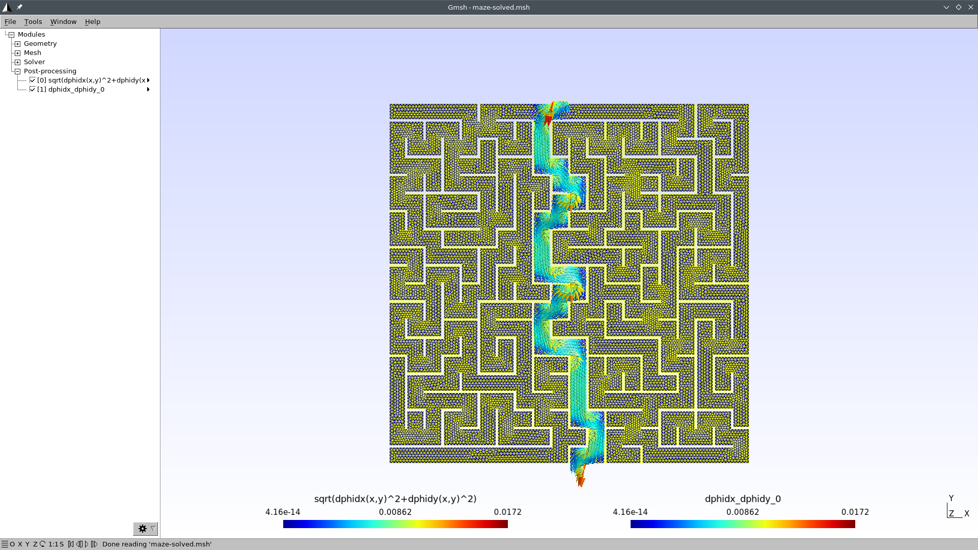
I bet you did not see the straightforward path that FeenoX found! Now
we just need some make up to make a nice social-network-worth picture.
Let us create a file maze-fig.geo so Gmsh can scale
everything up for us:
Merge "maze-solved.msh";

Mesh.SurfaceFaces = 0;
Mesh.SurfaceEdges = 0;
General.SmallAxes = 0;

General.GraphicsHeight = 940;
General.GraphicsWidth = 1380;

View[0].ShowScale = 0;
View[0].RangeType = 2;
View[0].CustomMax = 0.008;
View[0].SaturateValues = 1;


View[1].ShowScale = 0;
View[1].CustomMax = 1e-2;
View[1].RangeType = 2;
View[1].GlyphLocation = 1; // Glyph (arrow, number, etc.) location (1: center of gravity, 2: node)
View[1].ArrowSizeMax = 20;

Print "maze-solved.png";
Exit;
$ gmsh maze-fig.geo
$
5 Transient Laplace
Use this transient input file for FeenoX, with the same mesh, to
solve for the transient Laplace problem going from top to down
(i.e. td):
\nabla^2 \phi = \alpha \frac{\partial \phi}{\partial t}
PROBLEM laplace 2D
READ_MESH maze.msh

phi_0(x,y) = 0              # initial condition
end_time = 500              # some end time where we know we reached the steady-state
alpha = 1e-3                # factor of the time derivative to make it advance faster
BC start   phi=if(t<1,t,1)  # a ramp from zero to avoid discontinuities with the initial condition
BC end     phi=0            # homogeneous BC at the end (so we move from top to bottom)

SOLVE_PROBLEM
# PRINT t

# WRITE_MESH maze-tran-td.msh phi sqrt(dphidx(x,y)^2+dphidy(x,y)^2) VECTOR -dphidx(x,y) -dphidy(x,y) 0
$ feenox maze-tran-td.fee
0
0.00736111
0.017873
0.0338879
0.0541553
[...]
390.125
419.195
450.667
475.333
500
$So we have transient data in maze-tran-td.msh. Let’s
create a video (or a GIF) out of it. Use this
maze-tran-td-anim.geo to create PNGs of each time step:
Merge "maze-tran-td.msh";

Mesh.SurfaceFaces = 0;
Mesh.SurfaceEdges = 0;
General.SmallAxes = 0;

General.GraphicsHeight = 1024;
General.GraphicsWidth = General.MenuWidth + 1024;

View[0].Visible = 0;

View[1].ShowScale = 0;
View[1].RangeType = 2;
View[1].CustomMax = 0.01;
View[1].SaturateValues = 1;


View[2].ShowScale = 0;
View[2].CustomMax = 0.005;
View[2].RangeType = 2;
View[2].GlyphLocation = 1; // Glyph (arrow, number, etc.) location (1: center of gravity, 2: node)
View[2].ArrowSizeMax = 20;

For step In {0:View[0].NbTimeStep-1}
  View[1].TimeStep = step;
  View[2].TimeStep = step;
  Print Sprintf("maze-tran-td-%03g.png", step);
  Draw;
EndFor

General.Terminal = 1;
Printf("# all frames dumped, now run");
Printf("ffmpeg -y -framerate 10 -f image2 -i maze-tran-td-%%03d.png maze-tran-td.mp4");
Printf("ffmpeg -y -framerate 10 -f image2 -i maze-tran-td-%%03d.png maze-tran-td.gif");
Exit;
$ gmsh maze-tran-td-anim.geo
# all frames dumped, now run
ffmpeg -y -framerate 10 -f image2 -i maze-tran-td-%03d.png maze-tran-td.mp4
ffmpeg -y -framerate 10 -f image2 -i maze-tran-td-%03d.png maze-tran-td.gif
$ sudo apt-get install ffmpeg
[...]
$ ffmpeg -y -framerate 10 -f image2 -i maze-tran-td-%03d.png maze-tran-td.mp4
[...]
$ ffmpeg -y -framerate 10 -f image2 -i maze-tran-td-%03d.png maze-tran-td.gif
[...]
$
6 Homework
- Solve the bottom-up case.
- Play with different types of mazes! What if you actually draw and scan one yourself?
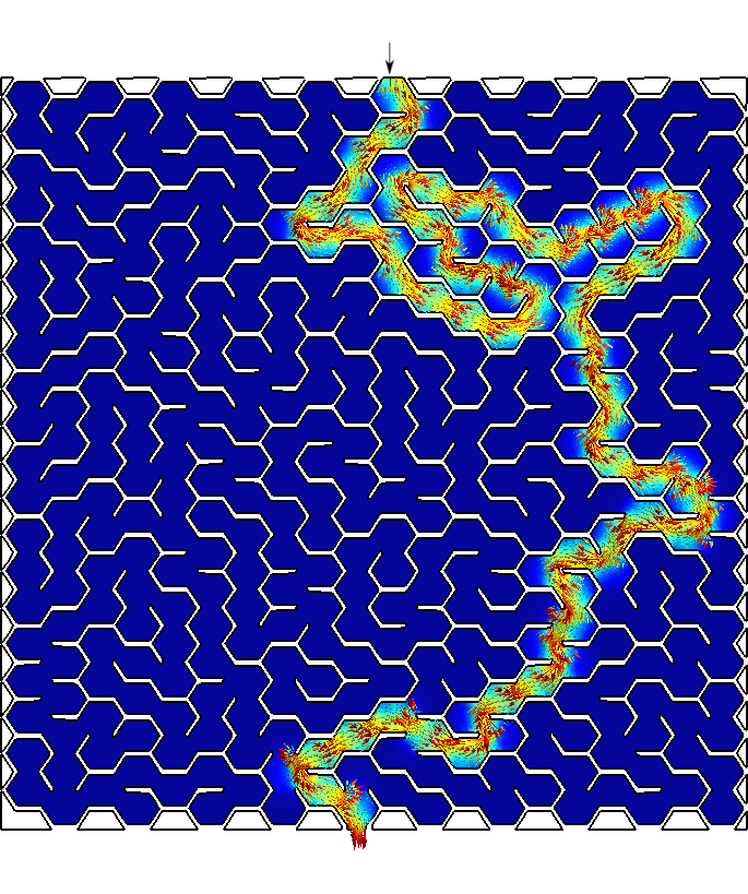
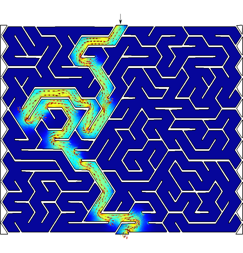
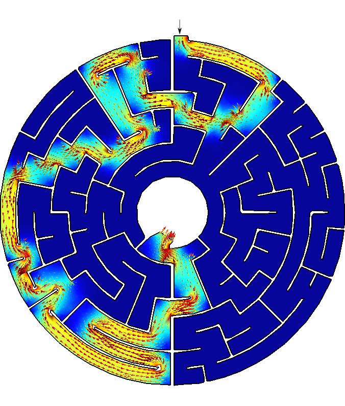
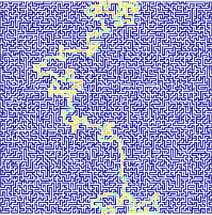
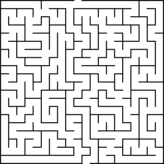
Figure 3: Any arbitrary maze (even hand-drawn) can be solved with FeenoX.