Laplace’s equation
Table of contents
1 How to solve a maze without AI
See these LinkedIn posts to see some comments and discussions:
- https://www.linkedin.com/feed/update/urn:li:activity:6831291311832760320/
- https://www.linkedin.com/feed/update/urn:li:activity:6973982270852325376/
Other people’s maze-related posts:
- https://www.linkedin.com/feed/update/urn:li:activity:6972370982489509888/
- https://www.linkedin.com/feed/update/urn:li:activity:6972949021711630336/
- https://www.linkedin.com/feed/update/urn:li:activity:6973522069703516160/
- https://www.linkedin.com/feed/update/urn:li:activity:6973921855275458560/
- https://www.linkedin.com/feed/update/urn:li:activity:6974663157952745472/
- https://www.linkedin.com/feed/update/urn:li:activity:6974979951049519104/
- https://www.linkedin.com/feed/update/urn:li:activity:6982049404568449024/
- https://www.linkedin.com/feed/update/urn:li:activity:6982049404568449024/
- https://www.linkedin.com/feed/update/urn:li:activity:7206676495879028736/
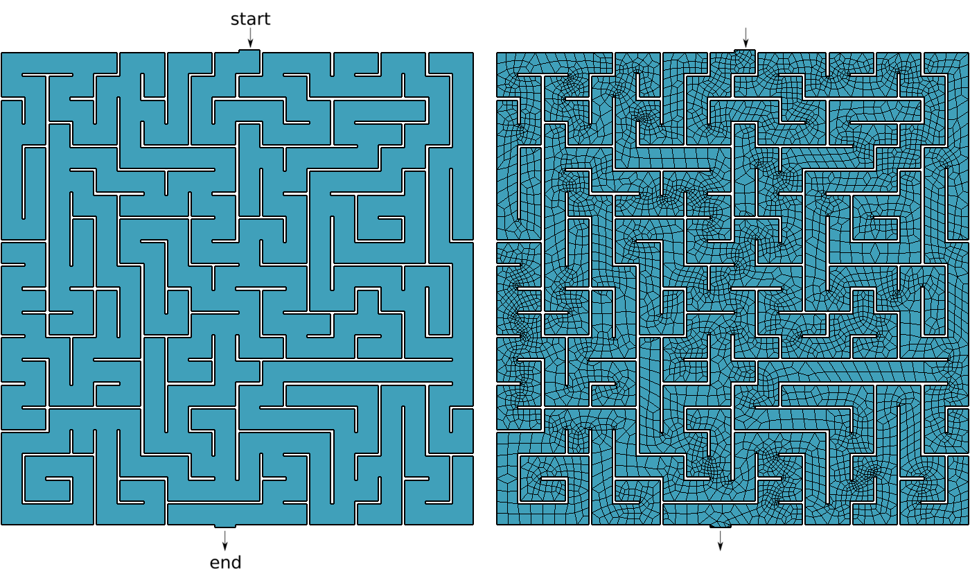
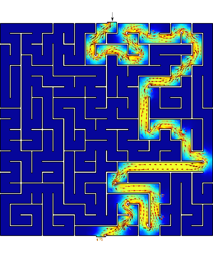
Say you are Homer Simpson and you want to solve a maze drawn in a restaurant’s placemat, one where both the start and end are known beforehand. In order to avoid falling into the alligator’s mouth, you can exploit the ellipticity of the Laplacian operator to solve any maze (even a hand-drawn one) without needing any fancy AI or ML algorithm. Just FeenoX and a bunch of standard open source tools to convert a bitmapped picture of the maze into an unstructured mesh.
PROBLEM laplace 2D  # pretty self-descriptive, isn't it?
READ_MESH maze.msh

# boundary conditions (default is homogeneous Neumann)
BC start  phi=0
BC end    phi=1

SOLVE_PROBLEM

# write the norm of gradient as a scalar field
# and the gradient as a 2d vector into a .msh file
WRITE_MESH maze-solved.msh \
    sqrt(dphidx(x,y)^2+dphidy(x,y)^2) \
    VECTOR dphidx dphidy 0
$ gmsh -2 maze.geo
[...]
$ feenox maze.fee
$
1.1 Transient top-down
Instead of solving a steady-state en exploiting the ellipticity of Laplace’s operator, let us see what happens if we solve a transient instead.
PROBLEM laplace 2D
READ_MESH maze.msh

phi_0(x,y) = 0              # initial condition
end_time = 100              # some end time where we know we reached the steady-state
alpha = 1e-6                # factor of the time derivative to make it advance faster
BC start   phi=if(t<1,t,1)  # a ramp from zero to avoid discontinuities with the initial condition
BC end     phi=0            # homogeneous BC at the end (so we move from top to bottom)

SOLVE_PROBLEM
PRINT t

WRITE_MESH maze-tran-td.msh phi    sqrt(dphidx(x,y)^2+dphidy(x,y)^2) VECTOR -dphidx(x,y) -dphidy(x,y) 0
WRITE_RESULTS
$ feenox maze-tran-td.fee
0
0.00433078
0.00949491
0.0170774
0.0268599
[...]
55.8631
64.0819
74.5784
87.2892
100
$ gmsh maze-tran-td-anim.geo
# all frames dumped, now run
ffmpeg -y -framerate 20 -f image2 -i maze-tran-td-%03d.png maze-tran-td.mp4
ffmpeg -y -framerate 20 -f image2 -i maze-tran-td-%03d.png maze-tran-td.gif
$ ffmpeg -y -framerate 20 -f image2 -i maze-tran-td-%03d.png maze-tran-td.mp4
[...]
$ ffmpeg -y -framerate 20 -f image2 -i maze-tran-td-%03d.png maze-tran-td.gif
[...]
1.2 Transient bottom-up
Now let us see what happens if we travel the maze from the exit up to the inlet. It looks like the solver tries a few different paths that lead nowhere until the actual solution is found.
PROBLEM laplace 2D
READ_MESH maze.msh

phi_0(x,y) = 0
end_time = 100
alpha = 1e-6
BC end     phi=if(t<1,t,1)
BC start   phi=0

SOLVE_PROBLEM
PRINT t

WRITE_MESH maze-tran-bu.msh phi    sqrt(dphidx(x,y)^2+dphidy(x,y)^2) VECTOR -dphidx(x,y) -dphidy(x,y) 0
WRITE_RESULTS
$ feenox maze-tran-bu.fee
0
0.00402961
0.00954806
0.0180156
0.0285787
[...]
65.3715
72.6894
81.8234
90.9117
100
$ gmsh maze-tran-bu-anim.geo
# all frames dumped, now run
ffmpeg -y -framerate 20 -f image2 -i maze-tran-bu-%03d.png maze-tran-bu.mp4
ffmpeg -y -framerate 20 -f image2 -i maze-tran-bu-%03d.png maze-tran-bu.gif
$ ffmpeg -y -framerate 20 -f image2 -i maze-tran-bu-%03d.png maze-tran-bu.mp4
[...]
$ ffmpeg -y -framerate 20 -f image2 -i maze-tran-bu-%03d.png maze-tran-bu.gif
[...]

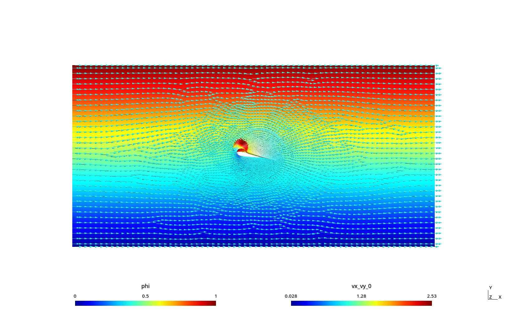
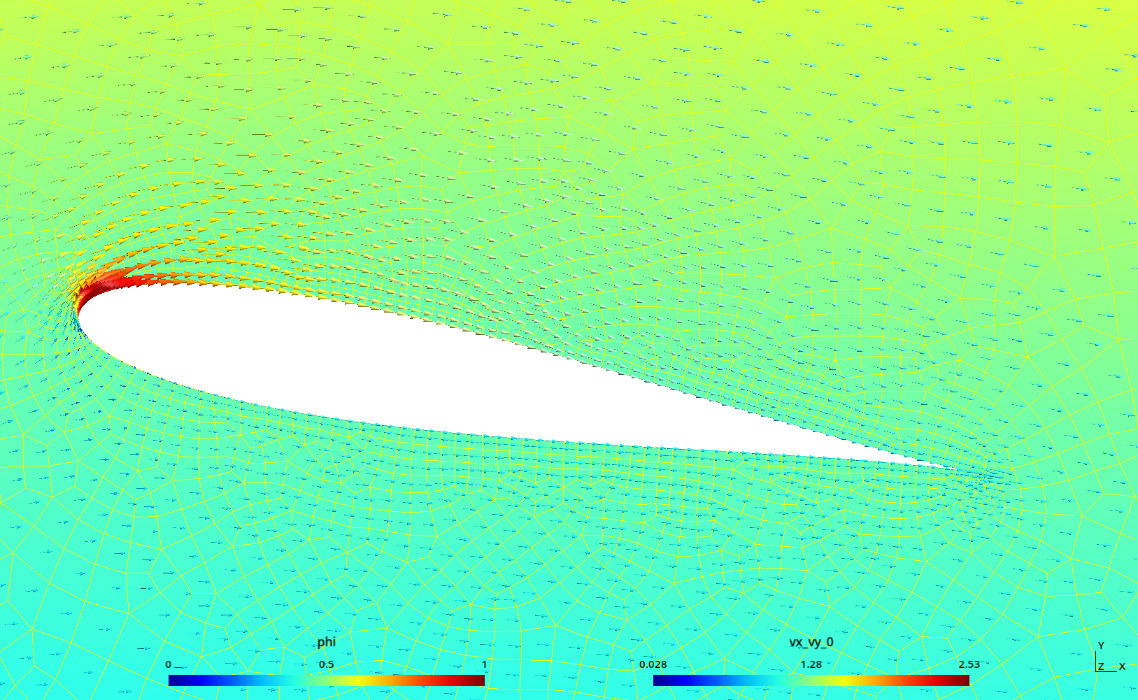
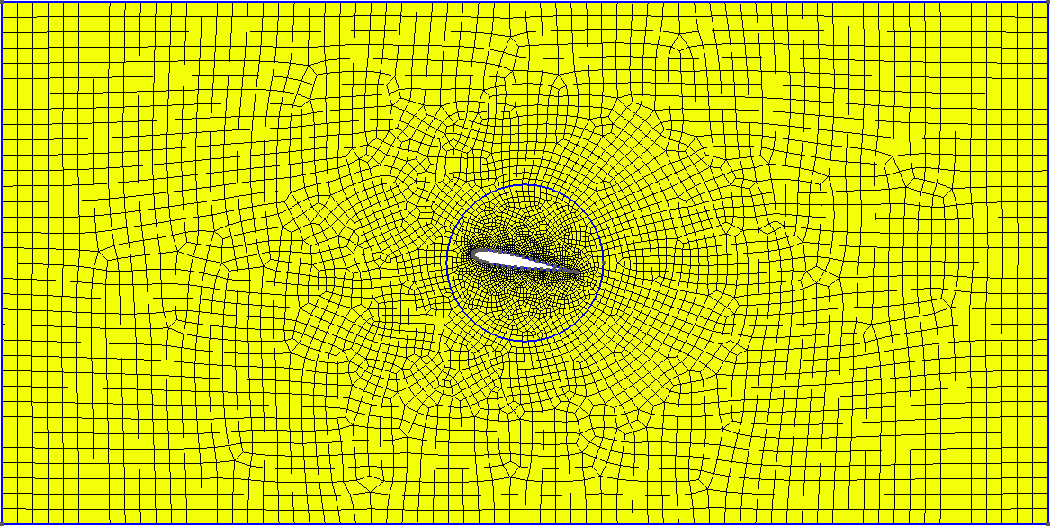
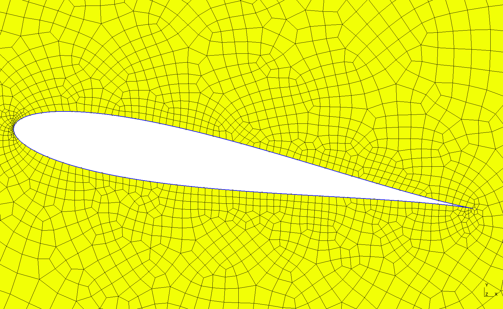
2 Potential flow around an airfoil profile
The Laplace equation can be used to model potential flow, as illustrated with this example from Prof. Enzo Dari for his course “Fluid Mechanics” at Instituto Balseiro.
For the particular case of a airfoil profile, the Dirichlet condition at the wing has to satisfy the Kutta condition.
This example
- Creates a symmetric airfoil-like Joukowsky profile using the the Gmsh Python API
- Solves the steady-state 2D Laplace equation with a different
Dirichlet value at the airfoil until the solution \phi evaluated at the continuation of the
wing tip matches the boundary value c.
It then computes the circulation integral of the velocities
- over the profile itself
- over a circle around the airfoil, computing the unitary tangential
vector
- from the internal normal variables
nxandny - from two functions
txandtyusing the circle’s equation
- from the internal normal variables
- around the original rectangular domain
nxandnzover the circle, respectively.
import sys
import math
import cmath
import gmsh

gmsh.initialize()

# size of the domain [-a,+a]x[-b,+b]
a = 20
b = 10

# characteristic element sizes
lc0 = 0.6       # near the boundary
lc = 0.1*lc0    # near the wing

# number of points of definition
nperf = 50
# attack angle
alpha = (float(sys.argv[1]) if len(sys.argv) > 1 else 10) * math.pi/180

# Joukowsky parameters
x0 = (float(sys.argv[2]) if len(sys.argv) > 2 else -0.11)
y0 = 0
r = math.sqrt((x0-1)**2+y0**2)

# append points
pts = []
coords = []
for i in range(nperf):
  theta = i * 2*math.pi/nperf
  dz = complex(x0 + r*math.cos(theta), y0 + r*math.sin(theta))
  z = (dz + 1/dz)*cmath.exp(complex(0, -alpha))
  # remember the coords of these three points
  if i == 0 or i == 1 or i == nperf-1:
    coords.append([z.real, z.imag])
  pts.append(gmsh.model.occ.addPoint(z.real, z.imag, 0, lc))

# create a closed loop of points
pts.append(pts[0])

# add a spline
spl = []
spl.append(gmsh.model.occ.addSpline(pts))
wing = gmsh.model.occ.addCurveLoop(spl)

# compute the location where to evaluate the Kutta condition
# this is ugly and not pythonic at all!
vsup = [-(coords[1][0] - coords[0][0]),
        -(coords[1][1] - coords[0][1])]
norm = math.sqrt(vsup[0]**2 + vsup[1]**2)
vsup[0] /= norm
vsup[1] /= norm

vinf = [-(coords[0][0] - coords[2][0]),
        -(coords[0][1] - coords[2][1])]
norm = math.sqrt(vinf[0]**2 + vinf[1]**2)
vinf[0] /= norm
vinf[1] /= norm

vmed = vsup + vinf
norm = math.sqrt(vmed[0]**2 + vmed[1]**2)
vmed[0] /= norm
vmed[1] /= norm

eps = 0.04
p = [coords[0][0] + eps * vmed[0],
     coords[0][1] + eps * vmed[1]]
# this is just to show the point in case one opens the .brep
kutta = gmsh.model.occ.addPoint(p[0], p[1], 0, lc)

# f = open("p.fee", "w")
# f.write( "VECTOR p[2] DATA %g %g\n" % (p[0], p[1]))
# f.close()


# add the external boundary
p1 = gmsh.model.occ.addPoint(-a, -b, 0, lc0)
p2 = gmsh.model.occ.addPoint(+a, -b, 0, lc0)
p3 = gmsh.model.occ.addPoint(+a, +b, 0, lc0)
p4 = gmsh.model.occ.addPoint(-a, +b, 0, lc0)
bottom   = gmsh.model.occ.addLine(p1, p2)
right    = gmsh.model.occ.addLine(p2, p3)
top      = gmsh.model.occ.addLine(p3, p4)
left     = gmsh.model.occ.addLine(p4, p1)
boundary = gmsh.model.occ.addCurveLoop([bottom, right, top, left])
air      = gmsh.model.occ.addPlaneSurface([boundary, wing])

# create a circle to compute the circulation
r_circle = 3
circle = gmsh.model.occ.addCircle(0, 0, 0, r_circle)


# we could embed the kutta point into the mesh but
# then the geometrical entities
ov, ovv = gmsh.model.occ.fragment([(2, air)], [(0, kutta), (1,circle)])
print(ov)
print(ovv)

gmsh.model.occ.synchronize()

# physical groups
# after the boolean fragment we lost the ids
# gmsh.model.addPhysicalGroup(1, [bottom], name="bottom")
# gmsh.model.addPhysicalGroup(1, [right],  name="right")
# gmsh.model.addPhysicalGroup(1, [top],    name="top")
# gmsh.model.addPhysicalGroup(1, [left],   name="left")
# gmsh.model.addPhysicalGroup(1, [wing],   name="wing")
# gmsh.model.addPhysicalGroup(2, [air],    name="air")

gmsh.model.addPhysicalGroup(0, [kutta], name="kutta")
gmsh.model.addPhysicalGroup(1, [6],     name="circle")
gmsh.model.addPhysicalGroup(1, [7],     name="bottom")
gmsh.model.addPhysicalGroup(1, [9],     name="right")
gmsh.model.addPhysicalGroup(1, [10],    name="top")
gmsh.model.addPhysicalGroup(1, [8],     name="left")
gmsh.model.addPhysicalGroup(1, [11],    name="wing")
gmsh.model.addPhysicalGroup(2, [1,2],   name="air")

# dump the brep (or xao) just in case
gmsh.write("airfoil.brep")
gmsh.write("airfoil.xao")


# mesh
gmsh.option.setNumber("Mesh.RecombineAll", 1)
gmsh.option.setNumber("Mesh.MeshSizeFromCurvature", 2*math.pi * 0.25 * r_circle/lc)
gmsh.option.setNumber("Mesh.Algorithm", 6)
gmsh.model.mesh.setAlgorithm(2, 1, 8);
gmsh.model.mesh.setAlgorithm(2, 2, 6);
gmsh.option.setNumber("Mesh.Smoothing", 10)

gmsh.model.mesh.generate(2)
gmsh.model.mesh.optimize("Netgen")
gmsh.model.mesh.optimize("Laplace2D")
gmsh.model.mesh.setOrder(2)
gmsh.model.mesh.optimize("HighOrderFastCurving")
gmsh.model.mesh.optimize("HighOrder")
gmsh.write("airfoil.msh")

# gmsh.fltk.run()
gmsh.finalize()
PROBLEM laplace 2D MESH airfoil.msh
static_steps = 20
# boundary conditions constant -> streamline
BC bottom phi=0
BC top phi=1
# initialize c = streamline constant for the wing
DEFAULT_ARGUMENT_VALUE 1 0.5
IF in_static_first
c = $1
ENDIF
BC wing phi=c
SOLVE_PROBLEM
PHYSICAL_GROUP kutta DIM 0
e = phi(kutta_cog[1], kutta_cog[2]) - c
PRINT TEXT "\# "step_static %.6f c %+.1e e HEADER
# check for convergence
done_static = done_static | (abs(e) < 1e-8)
IF done_static
PHYSICAL_GROUP left DIM 1
vx(x,y) = +dphidy(x,y) * left_length
vy(x,y) = -dphidx(x,y) * left_length
# write post-processing views
WRITE_MESH $0-converged.msh phi VECTOR vx vy 0
WRITE_MESH $0-converged.vtk phi VECTOR vx vy 0
# circulation on profile
INTEGRATE vx(x,y)*(+ny)+vy(x,y)*(-nx) OVER wing RESULT circ_profile
PRINTF "circ_profile = %g" -circ_profile
# function unit tangent
PHYSICAL_GROUP circle DIM 1
cx = circle_cog[1]
cy = circle_cog[2]
tx(x,y) = -(y-cy)/sqrt((x-cx)*(x-cx)+(y-cy)*(y-cy))
ty(x,y) = +(x-cx)/sqrt((x-cx)*(x-cx)+(y-cy)*(y-cy))
# circulation on the circumference with tangent
INTEGRATE vx(x,y)*tx(x,y)+vy(x,y)*ty(x,y) OVER circle RESULT circ_circle_t
PRINTF "circ_circle_t = %g" -circ_circle_t
# circulation on the outer box
INTEGRATE vx(x,y)*(+ny)+vy(x,y)*(-nx) OVER circle RESULT circ_circle_n
PRINTF "circ_circle_n = %g" -circ_circle_n
INTEGRATE -vx(x,y) OVER top GAUSS RESULT inttop
INTEGRATE +vx(x,y) OVER bottom GAUSS RESULT intbottom
INTEGRATE -vy(x,y) OVER left GAUSS RESULT intleft
INTEGRATE +vy(x,y) OVER right GAUSS RESULT intright
circ_box = inttop + intleft + intbottom + intright
PRINTF "circ_box = %g" -circ_box
# pressure forces
p(x,y) = 1.0 - vx(x,y)^2 + vy(x,y)^2
INTEGRATE p(x,y)*(nx) OVER circle RESULT pFx
PRINTF "pressure_drag = %g" pFx
INTEGRATE p(x,y)*(ny) OVER circle RESULT pFy
PRINTF "pressure_lift = %g" pFy
ELSE
# update c
IF in_static_first
c_last = c
e_last = e
c = c_last - 0.1
ELSE
c_next = c_last - e_last * (c_last-c)/(e_last-e)
c_last = c
e_last = e
c = c_next
ENDIF
ENDIF$ python airfoil.py
[...]
Info : Writing 'airfoil.msh'...
Info : Done writing 'airfoil.msh'
$ feenox airfoil.fee
# # step_static c e
# 1 0.500000 -3.4e-03
# 2 0.400000 +3.7e-03
# 3 0.452067 +2.0e-09
circ_profile = 2.49918
circ_circle_t = 2.49975
circ_circle_n = 2.49907
circ_box = 2.50379
pressure_drag = -0.00168068
pressure_lift = 2.60614
$